In last post we analyze the text of the U.S. constitution and its 27 amendments. Here we will generalize our analyze to many other countries.
On this website we can easily download the English version of constitution from 118 coutries using the following scripts:
import numpy as np
import urllib2
import matplotlib.pyplot as plt
import re
from bs4 import BeautifulSoup
import matplotlib.cm as cm
from collections import Counter
from sklearn.cluster import AffinityPropagation

def words(text): return re.findall('[a-z]+', text.lower())

def getConstitutionText():
    s='http://www.concourt.am/armenian/legal_resources/world_constitutions/constit/'
    url=s+'consts2l.htm'
    soup = BeautifulSoup(urllib2.urlopen(url).read())
    urls={}
    for a in soup.body.find_all('a', href=True):
        u = a['href']
        if u[-6:]=='-e.htm':
            if words(a.string)[0] == 'english' or words(a.string)[0] == 'in':
                urls[u.split('/')[0].title()]= s+u
            else:
                urls[words(a.string)[0].title()]= s+u
    W={}
    for key in urls:
        url=urls[key]
        d = re.sub('<[^<]+?>', '', urllib2.urlopen(url).read())
        d = words(d)
        W[key]=d
    return W

W = getConstitutionText()
Using the consine distance between text, we can derive a 116 x 116 matrix to represent the similarity between countries in terms of the content of consitution. Two cournties, Lithuania and UK, are removed due to a lack of data.
def cosine(i, k):
    i,k = map(lambda x:Counter(x), [i,k])
    q = set(i.keys()) & set(k.keys())
    a = sum([i[x] * k[x] for x in q])
    s1 = sum([i[x]**2 for x in i])
    s2 = sum([k[x]**2 for x in k])
    b = s1**0.5 * s2**0.5
    if not b:
        return 0.0
    else:
        return  float(a)/b

countries = W.keys()
countries = [i for i in countries if i!='Litva' and i!='Uk']
l=len(countries)
s = np.zeros(shape=(l,l))
for i in range(l):
    for j in range(l):
        s[i,j]=cosine(W[countries[i]],W[countries[j]])

plt.imshow(s)
plt.show()
The above scripts define the cosine distance, calculate the distance between courtries, and gives the plot below:
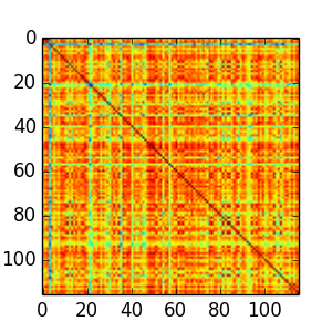
The values of the matrix cells varies from 0.707 to 1 (diagonal elements that represent the similarity between a constitution and itself). The most different consitutions in the data set are between Azerbaijan and Oceania (I am not sure this is a real country).
s.min()
from numpy import unravel_index
x,y = unravel_index(s.argmin(), s.shape)
countries[x],countries[y]
Using the Affinity Propagation algorithm, we can cluster the studies courties into 9 groups based on the cosine similarity matrix.
af = AffinityPropagation(preference=0.89, affinity="precomputed")
labels_precomputed = af.fit(s).labels_
#[[i,countries[j]] for i,j in enumerate(af.cluster_centers_indices_)]
dd = sorted(zip(countries,labels_precomputed),key=lambda x:x[1])
datatable=[['Country','Constitution Category']]
for i in dd:
    datatable.append([str(i[0].title()),i[1]])
len(set(labels_precomputed))
To display the results, we used the Geochart API provided by Google. In particular, we combined the clustering data of coutries with some fixed html scripts to generate a html page as follows:
htmla='''
<html>
  <head>
    <script type='text/javascript' src='https://www.google.com/jsapi'></script>
    <script type='text/javascript'>
     google.load('visualization', '1', {'packages': ['geochart']});
     google.setOnLoadCallback(drawRegionsMap);

      function drawRegionsMap() {
        var data = google.visualization.arrayToDataTable(
'''
htmlb='''
        );

        var options = {};
        options['dataMode'] = 'regions';
        options['colorAxis'] = { minValue : 0, maxValue : 8, colors :
        ['#011640','#2D5873','#7BA693','#E0542E','#BF9663','#684F2C','#F4A720','#EF8C12','#BFBA9F']};
        options['backgroundColor'] = '#FFFFFF';
        options['datalessRegionColor'] = '#E5E5E5';
        var chart = new google.visualization.GeoChart(document.getElementById('chart_div'));
        chart.draw(data, options);
    };
    </script>
  </head>
  <body>
    <div id="chart_div" style="width: 900px; height: 500px;"></div>
  </body>
</html>
'''
htmltext=htmla+str(datatable)+htmlb
open( "/Users/csid/Downloads/test.html", "w" ).write(htmltext)
If we open the generated html page, we see an interactive map, in which different countries are plotted in different colors. In writing this blog with markdown language, I took the advantage of this language and inseted the html scripts to display the above plot.
Some interesting assumptions can be obtained by observing the plot. There are courties which are close to each other in geological distance and also are similar with each other in terms of constitution. They are:
- China, Laos, and Vietnam (note that they are/were communist countries);
- Canada and the U.S. (The North America area);
- India and Pakistan (South Asia);
- East Europe countries including Russia.
I will leave more fun for the reader to discover more interesting things from this plot (such as the clusters in the middle east). But before we end this exploration, I would like to mention a surpring fact that is related to the current news in Crimea, Ukraine. Guess who is the only other country/region which share the similar constitutions with Ukraine in our data set?
Chechnya. You can not find this “country” in the above map because it is now already a part of Russia.