Master function and attention dynamics

2014-06-06 #network

Barabasi-Albert model

In their 1999 Science paper, Barabasi and Albert proposed the network model of preferential attachment. To obtain the degree distribution, they first used “continuous-time mean-field analysis” to track the evolution of the degree of individual nodes and then derive the degree distribution. In subsequent work, Dorogovstev, Mendes and Samukhin (2000), took a different approach, using what they call the “master equation” to obtain rigorous asymptotics for the mean degree of the nodes. The lecture note of Daron Acemoglu and Asu Ozdaglar to explain this method inspired me a lot to analyse the dynamics of attention networks.

First of all, let’s analyze BA model as a practice. We assume that

n is the number of nodes in the network; k is the degree of nodes; m is the fixed number of links carried by every newly added node; p_k is the fraction of nodes with degree k; and p_k,n is the fraction of nodes with degree k when there are n nodes in the network.

The probability of a new link attaches to a node of degree k is propotional to k/sum(k). This probability increases to

$\frac{k}{\sum_{k=1}^{k_{max}} k}n p_k = \frac{k}{\frac{1}{n}\sum_{k=1}^{k_{max}} k}p_k=\frac{k}{2m}p_k.\,\,\,\,\, (1)$

when we consider all nodes of degree k. If we consider the competition for the m links brought by a new node, we have

$m\frac{k}{2m}p_k= \frac{k}{2}p_k. \,\,\,\,\, (2)$

At each time step, the number of nodes with degree k changes. The change is composed by two parts: the increase contributed by the nodes moving from degree k-1 to k and and the loss caused by the nodes moving from degree k to k+1. Therefore we can express this change as:

$(n+1)p_{k,n+1}-np_{k,n} = \Delta k = \frac{k-1}{2}p_{k-1,n}-\frac{k}{2}p_{k,n}, \,\,\,\,\, (3)$

Eq.(3) hold when k > m. When k = m, there is no nodes moving from degree k-1 to k. The only possible increase of node number comes from the new node. So we revise the expression as

$(n+1)p_{m,n+1}-np_{m,n} = \Delta m = 1-\frac{m}{2}p_{m,n}, \,\,\,\,\, (4)$

Now, let’s assume that the system has envolved to such an equilibrium state that the degree distribution no more changes, i.e.,

$p_{k,n+1} = p_{k,n} = p_k, \,\,\,\,\, (5)$

then we have the function

$p_k = \frac{k-1}{2}p_{k-1}-\frac{k}{2}p_k, \,\,\,\,\, (k>m) (6)$

and

$p_m = 1-\frac{m}{2}p_m, \,\,\,\,\, (k=m), (7)$

from which we derive that

$\frac{p_k}{p_{k-1}} = \frac{k-1}{k+2} \,\,\,\,\, (k>m), (8)$

and

$p_m = \frac{2}{m+2} \,\,\,\,\, (k=m). (9)$

To solve p_k, we construct

$\frac{p_k}{p_m} = \frac{p_{m+1}}{p_{m}} ...\frac{p_{k-1}}{p_{k-2}}\frac{p_k}{p_{k-1}} \,\,\,\,\, (10)$

and find the solution

$p_k = \frac{2m(m+1)}{k(k+1)(k+2)}. \,\,\,\,\, (11)$

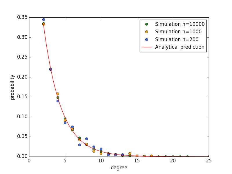
Eq.(11) approximates a power-law distribution with exponent equals -3 when k is large. This is the same as the result given by the 1999 paper.

The above figure shows the simulation of BA network with three different sizes. The degree distributions of nodes are always consistent with analytical prediction, independent of simulation size. The Python code for simulation is listed as follows:

import random
import networkx as nx
import matplotlib.pyplot as plt
import collections
import numpy as np
from os import listdir

# select random subset
def _random_subset(seq,m):
    targets=set()
    while len(targets)<m:
        x=random.choice(seq)
        targets.add(x)
    return targets
	
#BA model
def BA(n, m):
    G=nx.empty_graph(m)
    targets=list(range(m))
    repeated_nodes=[]
    source=m 
    while source<n: 
        G.add_edges_from(zip([source]*m,targets)) 
        repeated_nodes.extend(targets)
        repeated_nodes.extend([source]*m) 
        targets = _random_subset(repeated_nodes,m)
        source += 1
    return G

Growing random graph

Now let’s analyze a different network model. Everything is the same execpt that the new node randomly select m friends without considering their degrees.

The probability of a new link attaches to a node of degree k is propotional to 1/n. This probability increases to (1/n)np_k = p_k when we consider all nodes of degree k. If we consider the competition for the m links brought by a new node, we have m*p_k.

Similar to the BA model, we can derive that

$(n+1)p_{k,n+1}-np_{k,n} = \Delta k = mp_{k-1}-mp_k, \,\,\,\,\, (12)$

and

$(n+1)p_{m,n+1}-np_{m,n} = \Delta m = 1-mp_m. \,\,\,\,\, (13)$

Now, let’s focus on the stationary solutions of these euqations by considering Eq. (5):

$p_k = mp_{k-1}-mp_k, \,\,\,\,\, (k>m) (14)$

and

$p_m = 1-mp_m. \,\,\,\,\, (k=m), (15)$

from which we derive that

$\frac{p_k}{p_{k-1}} = \frac{m}{m+1} \,\,\,\,\, (k>m), (16)$

and

$p_m = \frac{1}{m+1} \,\,\,\,\, (k=m). (17)$

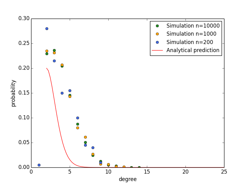
From Eq. (16), we find that the ratio of two fractions is independent of degree k, this is true because in our randomly growing network, new nodes do not consider the degree of existed nodes in setting up links. To solve p_k, we construct Eq. (10) again and find the solution

$p_k = \frac{1}{m+1}(\frac{m}{m+1})^{k-m}. \,\,\,\,\, (18)$

The above figure shows the simulation of random growing network with three different sizes. The degree distributions of nodes are always consistent with analytical prediction, independent of simulation size. The Python code for simulation is listed as follows:

#random network model
def ranG(n, m):
    G=nx.empty_graph(m)
    targets=list(range(m))
    unique_nodes=set()
    source=m 
    while source<n: 
        G.add_edges_from(zip([source]*m,targets))
        unique_nodes.update(targets)
        unique_nodes.add(source) 
        targets = _random_subset(list(unique_nodes),m)
        source += 1
    return G

Reversed BA model

Now let’s consider a “reversed” verion of the BA model, i.e., the probability of obtaining new links is proportional to the reciprocal of degree 1/k.

We assume that

$\sum_{i=1}^{n} \frac{1}{k} \approx n\frac{1}{2m}. \,\,\,\,\, (19)$

Then the probability of m new link attaches to nodes of degree k is

$\frac{\frac{1}{k}}{\sum_{i=1}^{n} \frac{1}{k}} np_k m \approx \frac{2m^2}{k}p_k. \,\,\,\,\, (20)$

Considering the stationary solution

$(n+1)p_{k,n+1}-np_{k,n} = \Delta k = p_k = A - B \approx\frac{2m^2}{k}p_k-\frac{2m^2}{k-1}p_{k-1}, \,\,\,\,\, (21)$

and

$(n+1)p_{m,n+1}-np_{m,n} = \Delta m = p_m = 1 - B = 1-\frac{2m^2}{m}p_{m}, \,\,\,\,\, (22)$

which leads to

$\frac{p_k}{p_{k-1}}=\frac{k}{k-1}\frac{2m^2}{k+2m^2}, \,\,\,\,\, (23)$

and

$p_m = \frac{1}{1 + 2m}. \,\,\,\,\, (24)$

As m is usually a small number (m=2 in classic BA model), when k is very large, we assume 2m^2/(k+2m^2) approximate 1/k to get

$\frac{p_k}{p_{k-1}} \sim \frac{1}{k-1}, \,\,\,\,\, (25)$

which gives

$p_k \approx \frac{1}{1 + m} \frac{1}{m(m+1)(m+2)...(k-1)}=\frac{1}{1 + 2m}\frac{(m-1)!}{(k-1)!}=\frac{1}{1 + m}\frac{e^{ln[(m-1)!]}}{e^{ln[(k-1)!]}}, \,\,\,\,\, (26)$

According to Stirling’s approximation,

$ln(n!) \approx nln(n) - n. \,\,\,\,\, (27)$

So we have

$p_k \approx \frac{1}{1 + 2m} \frac{(m-1)^{m-1}}{(k-1)^{k-1}}e^{k-m}, \,\,\,\,\, (27)$

In particular, when m = 2, p_k = (k-1)^(1-k) * e^(k-2) *1/5.

The above figure shows the simulation of revsered BA networks of three different sizes. The degree distributions of nodes are always consistent with analytical prediction, independent of simulation size. The Python code for simulation is listed as follows:

#weighted choice
def weighted_choice_sub(weights):
    rnd = random.random() * sum(weights)
    for i, w in enumerate(weights):
        rnd -= w
        if rnd < 0:
            return i

#weighted selection
def weightedDegreeSelection(nodeOccurance,m,gamma):
    c = collections.Counter(nodeOccurance)
    w = np.array(c.values())**float(gamma)
    s = [c.keys()[j] for j in [weighted_choice_sub(w) for i in range(m)]]
    return s

#reverse BA model
def rBA(n, m):
    G=nx.empty_graph(m)
    targets=list(range(m))
    repeated_nodes=[]
    source=m 
    while source<n: 
        G.add_edges_from(zip([source]*m,targets)) 
        repeated_nodes.extend(targets)
        repeated_nodes.extend([source]*m) 
        targets = weightedDegreeSelection(repeated_nodes,m,-1)
        source += 1
    return G

Mixture between random graph and BA model

Now we assume that a new node chooses a random friend with probability alpha and choose a friend with high degree with a probability 1-alpha.

Within the new m links, the following number of links are obtained by all nodes of degree k:

$(\alpha \frac{1}{n} + (1-\alpha) \frac{k}{\sum k}) n p_k m = (\alpha m +\frac{1-\alpha}{2}k)p_k, \,\,\,\,\, (28)$

We can derive that

$\frac{p_k}{p_{k-1}} = \frac{2 \alpha m + (1-\alpha)(k-1)}{2 + 2 \alpha m +(1-\alpha)k} = 1- \frac{3-\alpha}{2+2\alpha m + (1-\alpha)k}\,\,\,\,\, (29)$

and

$p_m = \frac{1}{1+\frac{1+\alpha}{2}m} \,\,\,\,\, (30)$

When k is very large, 2 + 2 alpha m is small compared to (1-alpha)k, so we can write Eq. (29) as

$\frac{p_k}{p_{k-1}} \approx 1- \frac{3-\alpha}{1-\alpha} \frac{1}{k} \approx (1-\frac{1}{k})^{\frac{3-\alpha}{1-\alpha}}=\frac{k}{k-1}^{-\frac{3-\alpha}{1-\alpha}}\,\,\,\,\, (31)$

By unfolding p_k/p_m as a long series like Eq. (10), we derive that

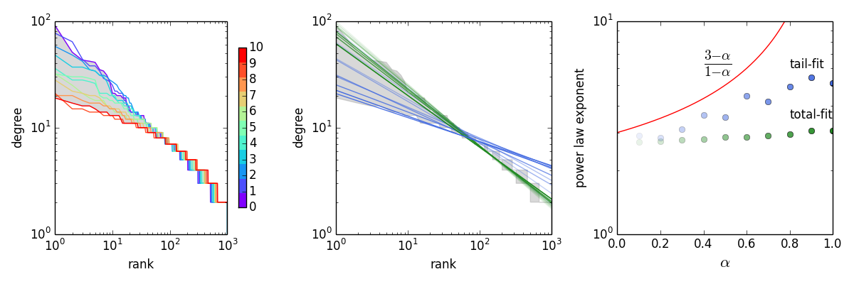
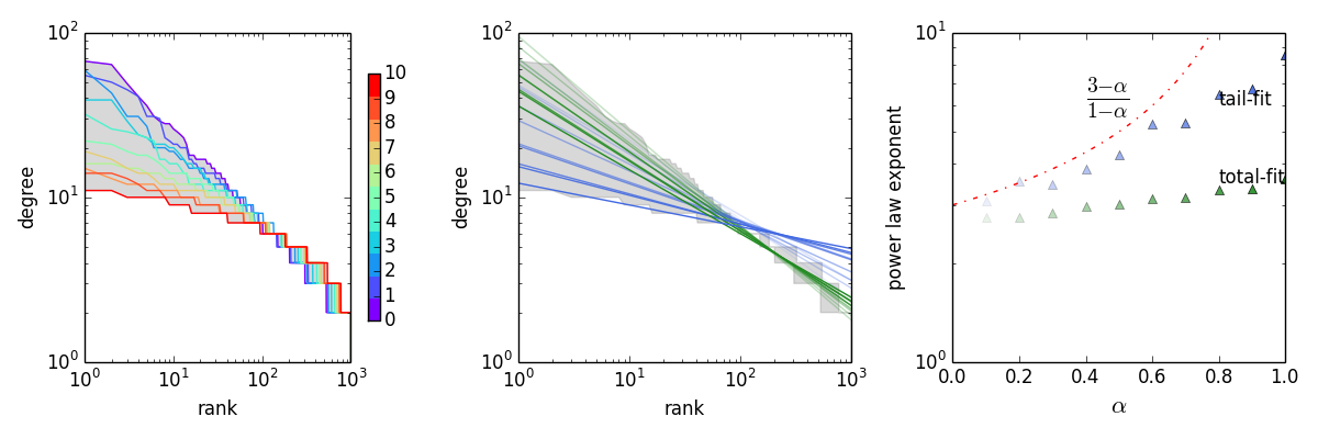
$p_k \approx \frac{1}{1+\frac{1+\alpha}{2}m} \frac{k}{m}^{-\frac{3-\alpha}{1-\alpha}} \,\,\,\,\, (30)$

mxedRandomBA

The above figure shows (1) the rank-order plot of mixture model when 10*alpha changes from 0 to 10; (2) the OLS fitting of the zipf exponent in log-log axes by total data (blue lines) and tail data (the largest 100 values, green lines). The tail fitting is better because when alpha is large, the distribution only approximates power-law in the tail. (3) The empirical values of power law exponent vs. alpha in two kinds of fittings and the thoretical curve (red line). Note that we fitted the data using rank-order plot (zipf-like), so we need to convert the fitted parameter b into 1+1/b in order to obatin power-law exponent. It turns out that theoretical curve only describes the data when alpha is small. This makes sense because when alpha approaches 1 the power-law distribution degenerates into an exponential distribution (Eq. (18)).

Mixture between reversed BA and BA model

Now we assume that a new node chooses a low-degree friend with probability alpha and choose a high-degree friend with probability 1-alpha.

Within the new m links, the following number of links are obtained by all nodes of degree k:

$(\alpha\frac{\frac{1}{k}}{\sum \frac{1}{k}} + (1-\alpha) \frac{k}{\sum k}) n p_k m \approx (\alpha \frac{2m^2 }{k} +(1-\alpha)\frac{k}{2})p_k, \,\,\,\,\, (31)$

We can derive that

$\frac{p_k}{p_{k-1}} =\frac{\frac{2m^2\alpha}{k-1}+\frac{(1-\alpha)(k-1)}{2}}{1+\frac{2m^2\alpha}{k}+\frac{(1-\alpha)k}{2}},\,\,\,\,\, (32)$

and

$p_m = \frac{2}{3m\alpha+m+2}. \,\,\,\,\, (33)$

When k is very large, 2m^2alpha/(k-1) approximates 0, so we can write Eq. (33) as

$\frac{p_k}{p_{k-1}} \approx\frac{\frac{(1-\alpha)(k-1)}{2}}{1+\frac{(1-\alpha)k}{2}}=\frac{k-1}{k+\frac{2}{1-\alpha}}.\,\,\,\,\, (34)$

By unfolding p_k/p_m as a long series like Eq. (10), we derive that

$\frac{p_k}{p_m} =\frac{p_{m+1}}{p_m}\frac{p_{m+2}}{p_{m+1}}...\frac{p_{k-1}}{p_{k-2}}\frac{p_{k}}{p_{k-1}}=\frac{m}{m+1+\frac{2}{1-\alpha}}\frac{m+1}{m+2+\frac{2}{1-\alpha}}...\frac{k-2}{k-1+\frac{2}{1-\alpha}}\frac{k-1}{k+\frac{2}{1-\alpha}}=m(m+1)...\frac{1}{k-1+\frac{2}{1-\alpha}}\frac{1}{k+\frac{2}{1-\alpha}},\,\,\,\,\, (35)$

in which the number h of items containing k satisfying

$k+\frac{2}{1-\alpha}-h =k-1.\,\,\,\,\, (36)$

This is because the numerator of the last item is k-1, and k only takes positive integers, so after going back for h items, k-h+2/(1-alpha) will eventually euqals k-1. Then the entire list will cancel out, only remaining the first h numerators containing m and the last denominators containing k. So the power law distribution has an exponent approximating -h. From Eq. (36) we derive that

$h = \frac{3-\alpha}{1-\alpha},\,\,\,\,\, (37)$

So the distribution can be written as

$p_k\approx\frac{2m^{\frac{3-\alpha}{1-\alpha}}}{3m\alpha+m+2}k^{-\frac{3-\alpha}{1-\alpha}}.\,\,\,\,\, (38)$

The following figure demonstrate that the analytical prediction is confirmed by simulation.

mxedreverseBA

The dynamics of collective attention in answering questions

A successful Q&A community should balance between answer quality and question coverage. This trade-off is constrained by the limitation of collective attention. To answer difficult/controversial questions, the community must “focus”. Meanwhile, to imporve the coverage rate, the community has to assign attention equaly among questions.

We suggest that the studed StackOverflow (SO) community archive this balance by allowing two different strategies at the individual level. The contributors of SO can be divided into two groups, “elephants” and “rats”. The former tends to embrace competition in answer questions whereas the latter tends to avoid competitions.

If we construct clickstream networks in which nodes are questions and links are user’s succesive answering of questions, these two different stragtegies correspond to two network growth mechanims. In particular, “elephant” strategy corresponds to BA model and “rat” strategy corresponds to the revsered BA model.

We show that, a mixture of BA and revsered BA with a ratio of 7:3, successfully replicates the distribution of answers across 10381 questions (the cumulative data in 50 days) in the Stackoverflow dataset, as shown by the following figure.

networks

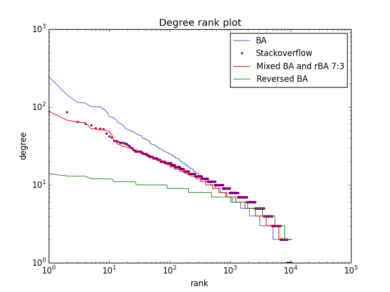
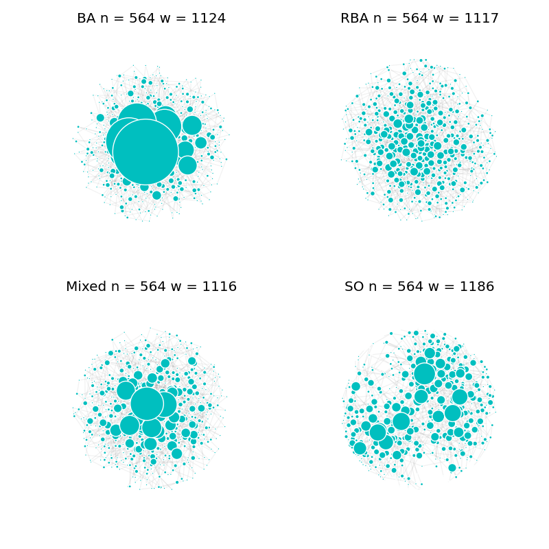
The above figure shows three different types of machenisms. We also include the StackOverflow data set in the first 8 days for comparison. There are about 500 nodes and 1000 links in each network. Please note that the difference between the networks in terms of the distribution of degree (the size of node is propotional to the square of degree).