 Figure by Kyle Szostek
Some text of this blog is cited from here
Figure by Kyle Szostek
Some text of this blog is cited from here
A piece of codes as the metaphor of universe
import random

def f(n):
    m = 0;
    for i in range(n):
        r = random.choice([0,1])
        m += r
    return m
The above Python code generates n 0/1 values and sums them up. If we only focus on the output, we will have the following observation

As shown by the figure, the most likely result is n/2 (n=100 in this case), and n/2 - 1 or n/2 + 1 is also very likely to be observed. As the values deviate from n/2, they becomes very unlikely to be observed.
Why? Becuse outputs correspond to a different number of combinations. f(n)=0 or f(n)=n corresonds to only one combination: it requires all n variables to be 0 or 1. But f(n)=n/2 corresonds to n!/(n/2)! combinations. So it is easier for us to observe f(n)=n/2.
Generally, the number of the combinations lead to f(n)=k is
Simple and straighforward, right? This is our metaphor of universe.
Let’s call a combination of the n values, such as 100100 or 000000, a microstate. And we call the sum of these values a macrostate. Then the logrithmic value of the number of microstates corresponding to a given macrostate, is the Boltzmann’s entropy of the macrostate.
 Figure cited from here
The above figure shows the grave of one of the greatest scientist, Boltzmann, who hanged himself during an attack of depression in 1906.
To summarize we give the following figure.

Let’s call a combination of the n values, such as 100100 or 000000, a microstate. And we call the sum of these values a macrostate. Then the logrithmic value of the number of microstates corresponding to a given macrostate, is the Boltzmann’s entropy of the macrostate.
Information theory as the foudation of thermodynamics
Let’s consider a thermodynamics model. Six gas particles are put into a big container:
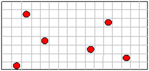
For simplicity we represent the container by a 2D grid containing 16*8 = 128 squares. So the total number of the microstate is 128^6. In the following graph we present 3 example microstates:

As discussed, we can also observe this system from the macroscopic level. The following figure shows the three macrostates corresponding to the above microstates.

We can also list all possible marcrostates and the number of microstates they correspond to

More generally, the number of combinations behind a macrostate is
in which n is the number of particles and g is the number of small squares (8 in our case) in a large square. The first items represents that the system is divide into two big squares, containing k and n-k particles, respectively. As both of g and n are constants, the value of omega only depends on the first item. In the following figure we plot the value of the first item against the the value of k.

As we can see, the value of the frst item, and hence the Boltzman entropy, is maximized when k=n/2. We also find that when the system size increases, the curve becomes sharp. It means that it is more likely to observed k=n/2 and more unlikelt to observe other macrostates. Finally, we should give the formal defnition of Boltzman entorpy as
The necessary of adding a constant coeffiecnt k_b = 1.38 * 10^-23 J/K is to make sure this formula comparible to Clausius entropy, which is defined on the macroscopic level of systems. This constant is also called Boltzman constant. Using this equation, Boltzmann, firstly in the histropy, gives microscopic exmplanations of the second law of thermodynamics, and hence pave way for a new area, statistical mechamics. The insight of Boltzmann is amazing, because when he wrote down the above formula, human beings were still not able to observe gas particles.
Entropy as the driven force of evolution
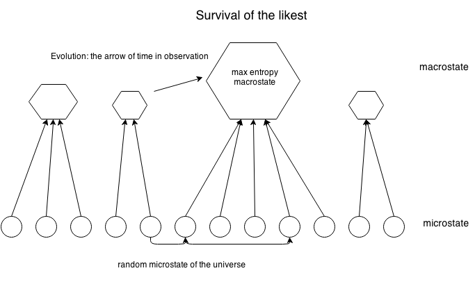
After briefly reviewing the history of entropy, we are prepared to think an interesting question: what is the driven force behind the evolution of complex systems ?
Entropy, as introduced, is the bridge connecting “microstates” and “macrostates”. Actcually, we can also understand it as the bridge connecting the “real-world” (which, may or may not exists, but we never know) and the “observed world”.
If we understand “observation” as a algorithm that ignores information, it may be easier for us to explain the arrow of time, and also the goal of evolution - the path and the goal are not determined by the system, but lies deeply in our “observation” algorithm.