君莫要逐云追梦

The definition of Ising model

_{Some of the following text come from here}

It is a simple model for a magnet where spins can point up or down, and like to align with their neighbours through a coupling constant J.

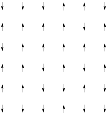
Energy describes the interactions between spins. The total energy of the system decreases for 1 unit if two connected spins have the same direction, and increases for 1 unit otherwise. We write the energy of the system as

in which J is a constant and the item following J sums over all connected pairs of spins. H represents the strength of the magnet field outside the system. The energy decreases 1 unit for every spin that has the same direction with the outside maget field.

Let’s see a concrete example, in which three spins are connected:

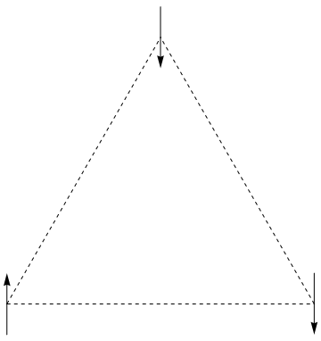
The system has 2^3 = 8 different states, including

We can calculate the energy for each of these states as

$E_{\{+1+1+1\}}=-J(1\times 1 + 1\times 1+ 1\times 1)-H(1+1+1)=-3J-3H, \,\,\,\,\, (3)$ $E_{\{+1+1-1\}}=-J((1\times 1)+(1\times (-1))+((-1)\times 1))-H(1+1-1)=J-H, \,\,\,\,\, (4)$ $E_{\{+1-1+1\}}=J-H, \,\,\,\,\, (5)$ $E_{\{+1-1-1\}}=J+H, \,\,\,\,\, (6)$ $E_{\{-1+1+1\}}=J-H, \,\,\,\,\, (7)$ $E_{\{-1+1-1\}}=J+H, \,\,\,\,\, (8)$ $E_{\{-1-1+1\}}=J+H, \,\,\,\,\, (9)$ $E_{\{-1-1-1\}}=-3J+3H, \,\,\,\,\, (10)$

and find that +1,+1,+1 is the state with minimum enegry.

Monte Carlo simulation

Different from agent-based models (ABM), in Ising model simulation we do not give rules for individual agents, but evolve the system according to some system-level statistics.

In particular, for each iteration, the program will randomly flip one spin. The new state s’ replaces old state s with a probability miu defined as

In other words, the old state will be remained with probability 1-miu. According to this rule, the system will have the following probability of state distribution

which is the famous Boltzmann distribution. k is the Boltzman constant = 1.3806488*10^{23}, and Z is the normalization factor

In statistical physics, Z is also called the partition function of system. It is the function of temperature T and maget field strength H.

See the following python code cited from here:

    #!/usr/bin/env python
"""
Monte Carlo simulation of the 2D Ising model
"""

from scipy import *
from scipy import weave
from pylab import *

Nitt = 1000000  # total number of Monte Carlo steps
N = 10          # linear dimension of the lattice, lattice-size= N x N
warm = 1000     # Number of warmup steps
measure=100     # How often to take a measurement


def CEnergy(latt):
    "Energy of a 2D Ising lattice at particular configuration"
    Ene = 0
    for i in range(len(latt)):
        for j in range(len(latt)):
            S = latt[i,j]
            WF = latt[(i+1)%N, j] + latt[i,(j+1)%N] + latt[(i-1)%N,j] + latt[i,(j-1)%N]
            Ene += -WF*S # Each neighbor gives energy 1.0
    return Ene/2. # Each par counted twice

def RandomL(N):
    "Radom lattice, corresponding to infinite temerature"
    latt = zeros((N,N), dtype=int)
    for i in range(N):
        for j in range(N):
            latt[i,j] = sign(2*rand()-1)
    return latt

def SamplePython(Nitt, latt, PW):
    "Monte Carlo sampling for the Ising model in Pythons"
    Ene = CEnergy(latt)  # Starting energy
    Mn=sum(latt)         # Starting magnetization
    
    Naver=0       # Measurements
    Eaver=0.0
    Maver=0.0
    
    N2 = N*N
    for itt in range(Nitt):
        t = int(rand()*N2)
        (i,j) = (t % N, t/N)
        S = latt[i,j]
        WF = latt[(i+1)%N, j] + latt[i,(j+1)%N] + latt[(i-1)%N,j] + latt[i,(j-1)%N]
        P = PW[4+S*WF]
        if P>rand(): # flip the spin
            latt[i,j] = -S
            Ene += 2*S*WF
            Mn -= 2*S
            
        if itt>warm and itt%measure==0:
            Naver += 1
            Eaver += Ene
            Maver += Mn

    return (Maver/Naver, Eaver/Naver)


def SampleCPP(Nitt, latt, PW, T):
    "The same Monte Carlo sampling in C++"
    Ene = float(CEnergy(latt))  # Starting energy
    Mn = float(sum(latt))       # Starting magnetization

    # Measurements
    aver = zeros(5,dtype=float) # contains: [Naver, Eaver, Maver]
    
    code="""
    using namespace std;
    int N2 = N*N;
    for (int itt=0; itt<Nitt; itt++){
        int t = static_cast<int>(drand48()*N2);
        int i = t % N;
        int j = t / N;
        int S = latt(i,j);
        int WF = latt((i+1)%N, j) + latt(i,(j+1)%N) + latt((i-1+N)%N,j) + latt(i,(j-1+N)%N);
        double P = PW(4+S*WF);
        if (P > drand48()){ // flip the spin
            latt(i,j) = -S;
            Ene += 2*S*WF;
            Mn -= 2*S;
        }
        if (itt>warm && itt%measure==0){
            aver(0) += 1;
            aver(1) += Ene;
            aver(2) += Mn;
            aver(3) += Ene*Ene;
            aver(4) += Mn*Mn;
        }
    }
    """
    weave.inline(code, ['Nitt','latt','N','PW','Ene','Mn','warm', 'measure', 'aver'],
                 type_converters=weave.converters.blitz, compiler = 'gcc')
    aE = aver[1]/aver[0]
    aM = aver[2]/aver[0]
    cv = (aver[3]/aver[0]-(aver[1]/aver[0])**2)/T**2
    chi = (aver[4]/aver[0]-(aver[2]/aver[0])**2)/T
    return (aM, aE, cv, chi)


if __name__ == '__main__':
    
    latt = RandomL(N)
    PW = zeros(9, dtype=float)

    wT = linspace(4,0.5,100)
    wMag=[]
    wEne=[]
    wCv=[]
    wChi=[]
    for T in wT:
        
        # Precomputed exponents
        PW[4+4] = exp(-4.*2/T)
        PW[4+2] = exp(-2.*2/T)
        PW[4+0] = exp(0.*2/T)
        PW[4-2] = exp( 2.*2/T)
        PW[4-4] = exp( 4.*2/T)
    
        #(maver, eaver) = SamplePython(Nitt, latt, PW)
        (aM, aE, cv, chi) = SampleCPP(Nitt, latt, PW, T)
        wMag.append( aM/(N*N) )
        wEne.append( aE/(N*N) )
        wCv.append( cv/(N*N) )
        wChi.append( chi/(N*N) )
        
        print T, aM/(N*N), aE/(N*N), cv/(N*N), chi/(N*N)
        
    plot(wT, wEne, label='E(T)')
    plot(wT, wCv, label='cv(T)')
    plot(wT, wMag, label='M(T)')
    xlabel('T')
    legend(loc='best')
    show()
    plot(wT, wChi, label='chi(T)')
    xlabel('T')
    legend(loc='best')
    show()

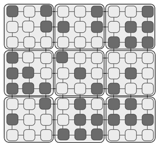
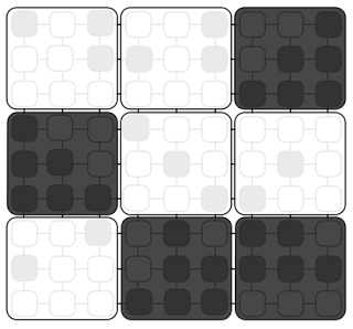
The following figure shows the result of simulation on a larger grid (than the one in the code)

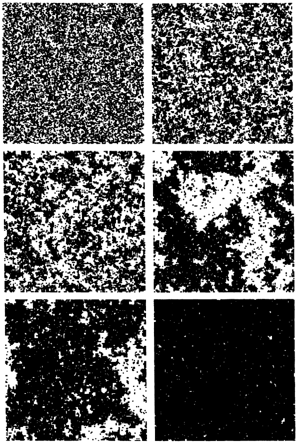
The first row shows T>Tc, the second row shows T~Tc, and the third row shows T<Tc.

Renormalization group

See the following figures cited from here:

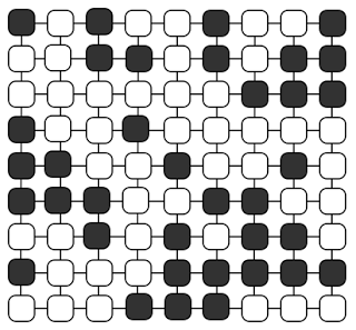
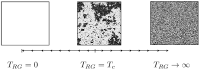
There is a striking feature of Ising model. When T ~ Tc, the strcuture of the grid is invariant of scale.

As shown by this video, when the temperature approaches the cirtical temperature, the information (of the ratio between the number of white and black spins) can not be compressed.